The main applications of factor analytic techniques are: (1) to reduce the number of variables and (2) to detect structure in the relationships between variables, that is to classify variables. Therefore, factor analysis is applied as a data reduction or structure detection method (the term factor analysis was first introduced by Thurstone, 1931). The topics listed below will describe the principles of factor analysis, and how it can be applied towards these two purposes. We will assume that you are familiar with the basic logic of statistical reasoning as described in Elementary Concepts. Moreover, we will also assume that you are familiar with the concepts of variance and correlation; if not, we advise that you read the Basic Statistics chapter at this point.
There are many excellent books on factor analysis. For example, a hands-on how-to approach can be found in Stevens (1986); more detailed technical descriptions are provided in Cooley and Lohnes (1971); Harman (1976); Kim and Mueller, (1978a, 1978b); Lawley and Maxwell (1971); Lindeman, Merenda, and Gold (1980); Morrison (1967); or Mulaik (1972). The interpretation of secondary factors in hierarchical factor analysis, as an alternative to traditional oblique rotational strategies, is explained in detail by Wherry (1984).
Confirmatory factor analysis. Structural Equation Modeling (SEPATH) allows you to test specific hypotheses about the factor structure for a set of variables, in one or several samples (e.g., you can compare factor structures across samples).
Correspondence analysis. Correspondence analysis is a descriptive/exploratory technique designed to analyze two-way and multi-way tables containing some measure of correspondence between the rows and columns. The results provide information which is similar in nature to those produced by factor analysis techniques, and they allow one to explore the structure of categorical variables included in the table. For more information regarding these methods, refer to Correspondence Analysis.
| To index |
Basic Idea of Factor Analysis as a Data Reduction Method
Suppose we conducted a (rather "silly") study in which we measure 100 people's height in inches and centimeters. Thus, we would have two variables that measure height. If in future studies, we want to research, for example, the effect of different nutritional food supplements on height, would we continue to use both measures? Probably not; height is one characteristic of a person, regardless of how it is measured.
Let us now extrapolate from this "silly" study to something that one might actually do as a researcher. Suppose we want to measure people's satisfaction with their lives. We design a satisfaction questionnaire with various items; among other things we ask our subjects how satisfied they are with their hobbies (item 1) and how intensely they are pursuing a hobby (item 2). Most likely, the responses to the two items are highly correlated with each other. (If you are not familiar with the correlation coefficient, we recommend that you read the description in Basic Statistics - Correlations) Given a high correlation between the two items, we can conclude that they are quite redundant.
Combining Two Variables into a Single Factor. One can summarize the correlation between two variables in a scatterplot. A regression line can then be fitted that represents the "best" summary of the linear relationship between the variables. If we could define a variable that would approximate the regression line in such a plot, then that variable would capture most of the "essence" of the two items. Subjects' single scores on that new factor, represented by the regression line, could then be used in future data analyses to represent that essence of the two items. In a sense we have reduced the two variables to one factor. Note that the new factor is actually a linear combination of the two variables.
Principal Components Analysis. The example described above, combining two correlated variables into one factor, illustrates the basic idea of factor analysis, or of principal components analysis to be precise (we will return to this later). If we extend the two-variable example to multiple variables, then the computations become more involved, but the basic principle of expressing two or more variables by a single factor remains the same.
Extracting Principal Components. We do not want to go into the details about the computational aspects of principal components analysis here, which can be found elsewhere (references were provided at the beginning of this section). However, basically, the extraction of principal components amounts to a variance maximizing (varimax) rotation of the original variable space. For example, in a scatterplot we can think of the regression line as the original X axis, rotated so that it approximates the regression line. This type of rotation is called variance maximizing because the criterion for (goal of) the rotation is to maximize the variance (variability) of the "new" variable (factor), while minimizing the variance around the new variable (see Rotational Strategies).
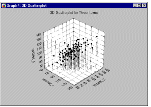
Generalizing to the Case of Multiple Variables. When there are more than two variables, we can think of them as defining a "space," just as two variables defined a plane. Thus, when we have three variables, we could plot a three- dimensional scatterplot, and, again we could fit a plane through the data.

With more than three variables it becomes impossible to illustrate the points in a scatterplot, however, the logic of rotating the axes so as to maximize the variance of the new factor remains the same.
Multiple orthogonal factors. After we have found the line on which the variance is maximal, there remains some variability around this line. In principal components analysis, after the first factor has been extracted, that is, after the first line has been drawn through the data, we continue and define another line that maximizes the remaining variability, and so on. In this manner, consecutive factors are extracted. Because each consecutive factor is defined to maximize the variability that is not captured by the preceding factor, consecutive factors are independent of each other. Put another way, consecutive factors are uncorrelated or orthogonal to each other.
How many Factors to Extract? Remember that, so far, we are considering principal components analysis as a data reduction method, that is, as a method for reducing the number of variables. The question then is, how many factors do we want to extract? Note that as we extract consecutive factors, they account for less and less variability. The decision of when to stop extracting factors basically depends on when there is only very little "random" variability left. The nature of this decision is arbitrary; however, various guidelines have been developed, and they are reviewed in Reviewing the Results of a Principal Components Analysis under Eigenvalues and the Number-of- Factors Problem.
Reviewing the Results of a Principal Components Analysis. Without further ado, let us now look at some of the standard results from a principal components analysis. To reiterate, we are extracting factors that account for less and less variance. To simplify matters, one usually starts with the correlation matrix, where the variances of all variables are equal to 1.0. Therefore, the total variance in that matrix is equal to the number of variables. For example, if we have 10 variables each with a variance of 1 then the total variability that can potentially be extracted is equal to 10 times 1. Suppose that in the satisfaction study introduced earlier we included 10 items to measure different aspects of satisfaction at home and at work. The variance accounted for by successive factors would be summarized as follows:
| STATISTICA FACTOR ANALYSIS |
Eigenvalues
(factor.sta) Extraction: Principal components | |||
|---|---|---|---|---|
| Value |
Eigenval |
% total Variance |
Cumul. Eigenval |
Cumul. % |
| 1 2 3 4 5 6 7 8 9 10 |
6.118369 1.800682 .472888 .407996 .317222 .293300 .195808 .170431 .137970 .085334 |
61.18369 18.00682 4.72888 4.07996 3.17222 2.93300 1.95808 1.70431 1.37970 .85334 |
6.11837 7.91905 8.39194 8.79993 9.11716 9.41046 9.60626 9.77670 9.91467 10.00000 |
61.1837 79.1905 83.9194 87.9993 91.1716 94.1046 96.0626 97.7670 99.1467 100.0000 |
Eigenvalues
In the second column (Eigenvalue) above, we find
the variance on the new factors that were successively extracted. In the third
column, these values are expressed as a percent of the total variance (in this
example, 10). As we can see, factor 1 accounts for 61 percent of the variance,
factor 2 for 18 percent, and so on. As expected, the sum of the eigenvalues is
equal to the number of variables. The third column contains the cumulative
variance extracted. The variances extracted by the factors are called the
eigenvalues. This name derives from the computational issues involved.
Eigenvalues and the Number-of-Factors Problem
Now that we have a
measure of how much variance each successive factor extracts, we can return to
the question of how many factors to retain. As mentioned earlier, by its nature
this is an arbitrary decision. However, there are some guidelines that are
commonly used, and that, in practice, seem to yield the best results.
The Kaiser criterion. First, we can retain only factors with eigenvalues greater than 1. In essence this is like saying that, unless a factor extracts at least as much as the equivalent of one original variable, we drop it. This criterion was proposed by Kaiser (1960), and is probably the one most widely used. In our example above, using this criterion, we would retain 2 factors (principal components).
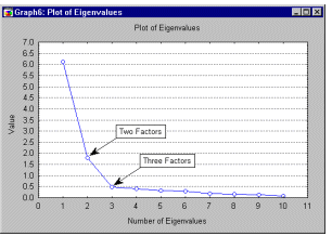
The scree test. A graphical method is the scree test first proposed by Cattell (1966). We can plot the eigenvalues shown above in a simple line plot.

Cattell suggests to find the place where the smooth decrease of eigenvalues appears to level off to the right of the plot. To the right of this point, presumably, one finds only "factorial scree" -- "scree" is the geological term referring to the debris which collects on the lower part of a rocky slope. According to this criterion, we would probably retain 2 or 3 factors in our example.
Which criterion to use. Both criteria have been studied in detail (Browne, 1968; Cattell & Jaspers, 1967; Hakstian, Rogers, & Cattell, 1982; Linn, 1968; Tucker, Koopman & Linn, 1969). Theoretically, one can evaluate those criteria by generating random data based on a particular number of factors. One can then see whether the number of factors is accurately detected by those criteria. Using this general technique, the first method (Kaiser criterion) sometimes retains too many factors, while the second technique (scree test) sometimes retains too few; however, both do quite well under normal conditions, that is, when there are relatively few factors and many cases. In practice, an additional important aspect is the extent to which a solution is interpretable. Therefore, one usually examines several solutions with more or fewer factors, and chooses the one that makes the best "sense." We will discuss this issue in the context of factor rotations below.
Principal Factors Analysis
Before we continue to examine the
different aspects of the typical output from a principal components analysis,
let us now introduce principal factors analysis. Let us return to our
satisfaction questionnaire example to conceive of another "mental model" for
factor analysis. We can think of subjects' responses as being dependent on two
components. First, there are some underlying common factors, such as the
"satisfaction-with-hobbies" factor we looked at before. Each item measures some
part of this common aspect of satisfaction. Second, each item also captures a
unique aspect of satisfaction that is not addressed by any other item.
Communalities. If this model is correct, then we should not expect that the factors will extract all variance from our items; rather, only that proportion that is due to the common factors and shared by several items. In the language of factor analysis, the proportion of variance of a particular item that is due to common factors (shared with other items) is called communality. Therefore, an additional task facing us when applying this model is to estimate the communalities for each variable, that is, the proportion of variance that each item has in common with other items. The proportion of variance that is unique to each item is then the respective item's total variance minus the communality. A common starting point is to use the squared multiple correlation of an item with all other items as an estimate of the communality (refer to Multiple Regression for details about multiple regression). Some authors have suggested various iterative "post-solution improvements" to the initial multiple regression communality estimate; for example, the so-called MINRES method (minimum residual factor method; Harman & Jones, 1966) will try various modifications to the factor loadings with the goal to minimize the residual (unexplained) sums of squares.
Principal factors vs. principal components. The defining characteristic then that distinguishes between the two factor analytic models is that in principal components analysis we assume that all variability in an item should be used in the analysis, while in principal factors analysis we only use the variability in an item that it has in common with the other items. A detailed discussion of the pros and cons of each approach is beyond the scope of this introduction (refer to the general references provided in Principal components and Factor Analysis - Introductory Overview). In most cases, these two methods usually yield very similar results. However, principal components analysis is often preferred as a method for data reduction, while principal factors analysis is often preferred when the goal of the analysis is to detect structure (see Factor Analysis as a Classification Method).
| To index |
Factor Analysis as a Classification Method
Let us now return to the interpretation of the standard results from a factor analysis. We will henceforth use the term factor analysis generically to encompass both principal components and principal factors analysis. Let us assume that we are at the point in our analysis where we basically know how many factors to extract. We may now want to know the meaning of the factors, that is, whether and how we can interpret them in a meaningful manner. To illustrate how this can be accomplished, let us work "backwards," that is, begin with a meaningful structure and then see how it is reflected in the results of a factor analysis. Let us return to our satisfaction example; shown below is the correlation matrix for items pertaining to satisfaction at work and items pertaining to satisfaction at home.
| STATISTICA FACTOR ANALYSIS |
Correlations
(factor.sta) Casewise deletion of MD n=100 | |||||
|---|---|---|---|---|---|---|
| Variable | WORK_1 | WORK_2 | WORK_3 | HOME_1 | HOME_2 | HOME_3 |
| WORK_1 WORK_2 WORK_3 HOME_1 HOME_2 HOME_3 |
1.00 .65 .65 .14 .15 .14 |
.65 1.00 .73 .14 .18 .24 |
.65 .73 1.00 .16 .24 .25 |
.14 .14 .16 1.00 .66 .59 |
.15 .18 .24 .66 1.00 .73 |
.14 .24 .25 .59 .73 1.00 |
Factor Loadings. Let us now perform a principal components analysis and look at the two-factor solution. Specifically, let us look at the correlations between the variables and the two factors (or "new" variables), as they are extracted by default; these correlations are also called factor loadings.
| STATISTICA FACTOR ANALYSIS |
Factor Loadings
(Unrotated) Principal components | |
|---|---|---|
| Variable | Factor 1 | Factor 2 |
| WORK_1 WORK_2 WORK_3 HOME_1 HOME_2 HOME_3 |
.654384 .715256 .741688 .634120 .706267 .707446 |
.564143 .541444 .508212 -.563123 -.572658 -.525602 |
| Expl.Var Prp.Totl |
2.891313 .481885 |
1.791000 .298500 |
Rotating the Factor Structure. We could plot the factor loadings shown above in a scatterplot. In that plot, each variable is represented as a point. In this plot we could rotate the axes in any direction without changing the relative locations of the points to each other; however, the actual coordinates of the points, that is, the factor loadings would of course change. In this example, if you produce the plot it will be evident that if we were to rotate the axes by about 45 degrees we might attain a clear pattern of loadings identifying the work satisfaction items and the home satisfaction items.
Rotational strategies. There are various rotational strategies that have been proposed. The goal of all of these strategies is to obtain a clear pattern of loadings, that is, factors that are somehow clearly marked by high loadings for some variables and low loadings for others. This general pattern is also sometimes referred to as simple structure (a more formalized definition can be found in most standard textbooks). Typical rotational strategies are varimax, quartimax, and equamax.
We have described the idea of the varimax rotation before (see Extracting Principal Components), and it can be applied to this problem as well. As before, we want to find a rotation that maximizes the variance on the new axes; put another way, we want to obtain a pattern of loadings on each factor that is as diverse as possible, lending itself to easier interpretation. Below is the table of rotated factor loadings.
| STATISTICA FACTOR ANALYSIS |
Factor Loadings
(Varimax normalized) Extraction: Principal components | |
|---|---|---|
| Variable | Factor 1 | Factor 2 |
| WORK_1 WORK_2 WORK_3 HOME_1 HOME_2 HOME_3 |
.862443 .890267 .886055 .062145 .107230 .140876 |
.051643 .110351 .152603 .845786 .902913 .869995 |
| Expl.Var Prp.Totl |
2.356684 .392781 |
2.325629 .387605 |
Interpreting the Factor Structure. Now the pattern is much clearer. As expected, the first factor is marked by high loadings on the work satisfaction items, the second factor is marked by high loadings on the home satisfaction items. We would thus conclude that satisfaction, as measured by our questionnaire, is composed of those two aspects; hence we have arrived at a classification of the variables.
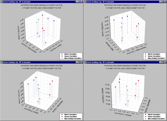
Consider another example, this time with four additional Hobby/Misc variables added to our earlier example.

In the plot of factor loadings above, 10 variables were reduced to three specific factors, a work factor, a home factor and a hobby/misc. factor. Note that factor loadings for each factor are spread out over the values of the other two factors but are high for its own values. For example, the factor loadings for the hobby/misc variables (in green) have both high and low "work" and "home" values, but all four of these variables have high factor loadings on the "hobby/misc" factor.
Oblique Factors. Some authors (e.g., Catell & Khanna; Harman, 1976; Jennrich & Sampson, 1966; Clarkson & Jennrich, 1988) have discussed in some detail the concept of oblique (non-orthogonal) factors, in order to achieve more interpretable simple structure. Specifically, computational strategies have been developed to rotate factors so as to best represent "clusters" of variables, without the constraint of orthogonality of factors. However, the oblique factors produced by such rotations are often not easily interpreted. To return to the example discussed above, suppose we would have included in the satisfaction questionnaire above four items that measured other, "miscellaneous" types of satisfaction. Let us assume that people's responses to those items were affected about equally by their satisfaction at home (Factor 1) and at work (Factor 2). An oblique rotation will likely produce two correlated factors with less-than- obvious meaning, that is, with many cross-loadings.
Hierarchical Factor Analysis. Instead of computing loadings for often difficult to interpret oblique factors, you can use a strategy first proposed by Thompson (1951) and Schmid and Leiman (1957), which has been elaborated and popularized in the detailed discussions by Wherry (1959, 1975, 1984). In this strategy, you first identify clusters of items and rotate axes through those clusters; next the correlations between those (oblique) factors is computed, and that correlation matrix of oblique factors is further factor-analyzed to yield a set of orthogonal factors that divide the variability in the items into that due to shared or common variance (secondary factors), and unique variance due to the clusters of similar variables (items) in the analysis (primary factors). To return to the example above, such a hierarchical analysis might yield the following factor loadings:
| STATISTICA FACTOR ANALYSIS |
Secondary & Primary
Factor Loadings | ||
|---|---|---|---|
| Factor | Second. 1 | Primary 1 | Primary 2 |
| WORK_1 WORK_2 WORK_3 HOME_1 HOME_2 HOME_3 MISCEL_1 MISCEL_2 MISCEL_3 MISCEL_4 |
.483178 .570953 .565624 .535812 .615403 .586405 .780488 .734854 .776013 .714183 |
.649499 .687056 .656790 .117278 .079910 .065512 .466823 .464779 .439010 .455157 |
.187074 .140627 .115461 .630076 .668880 .626730 .280141 .238512 .303672 .228351 |
Careful examination of these loadings would lead to the following conclusions:
Confirmatory Factor Analysis. Over the past 15 years, so-called confirmatory methods have become increasingly popular (e.g., see Jöreskog and Sörbom, 1979). In general, one can specify a priori, a pattern of factor loadings for a particular number of orthogonal or oblique factors, and then test whether the observed correlation matrix can be reproduced given these specifications. Confirmatory factor analyses can be performed via Structural Equation Modeling (SEPATH).
| To index |
Miscellaneous Other Issues and Statistics
Factor Scores. We can estimate the actual values of individual cases (observations) for the factors. These factor scores are particularly useful when one wants to perform further analyses involving the factors that one has identified in the factor analysis.
Reproduced and Residual Correlations. An additional check for the appropriateness of the respective number of factors that were extracted is to compute the correlation matrix that would result if those were indeed the only factors. That matrix is called the reproduced correlation matrix. To see how this matrix deviates from the observed correlation matrix, one can compute the difference between the two; that matrix is called the matrix of residual correlations. The residual matrix may point to "misfits," that is, to particular correlation coefficients that cannot be reproduced appropriately by the current number of factors.
Matrix Ill-conditioning. If, in the correlation matrix there are variables that are 100% redundant, then the inverse of the matrix cannot be computed. For example, if a variable is the sum of two other variables selected for the analysis, then the correlation matrix of those variables cannot be inverted, and the factor analysis can basically not be performed. In practice this happens when you are attempting to factor analyze a set of highly intercorrelated variables, as it, for example, sometimes occurs in correlational research with questionnaires. Then you can artificially lower all correlations in the correlation matrix by adding a small constant to the diagonal of the matrix, and then restandardizing it. This procedure will usually yield a matrix that now can be inverted and thus factor-analyzed; moreover, the factor patterns should not be affected by this procedure. However, note that the resulting estimates are not exact.
| To index |